
 Open this simulation and click on "charts." Move the man left and right to see how graphs correspond to motion.
In this section, you will look at how the equations in the previous section connect to graphs. Take a moment to look at the following simulation showing the relationship between one-dimensional motion and graphs.
Open this simulation and click on "charts." Move the man left and right to see how graphs correspond to motion.
Now let’s take a moment to look at some graphs representing real-world situations. Before beginning each scenario, look closely at the graph, and then return to the simulation to see if you can re-create the graph. Describe what is happening in your notes.
It is important to recognize some of the basic graphs associated with one-dimensional motion. The most common ones used by scientists are the displacement vs. time, velocity vs. time, and the acceleration vs. time. Let's start by looking at a displacement vs. time for someone riding her bike at a constant velocity.
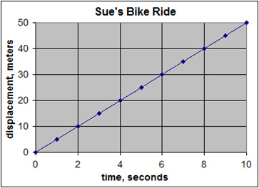
This graph shows that Sue's displacement during her bike ride is increasing along a straight line. The slope of this line (rise over run) is 5. This means that Sue's velocity is constant at 5 m/s. If the velocity were negative, the line would slope down.
For another example, assume that John starts at position d = 0 m, with velocity v = 0 m/s, and that he accelerates at 2 m/s2 for 10 seconds. What is his position and velocity at 5 s? Since John is accelerating at a constant rate, the associated graphs look a bit different than the graph of displacement vs. time at constant velocity. The acceleration vs. time graph looks like the following.
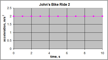
In the graph, the line is flat, which means the acceleration is constant. As you can see, the value of the acceleration is 2 m/s2.
Using the same situation, the graph of velocity vs. time looks like the following.
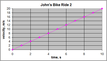
You can read right off the graph that John's velocity at 5 s is 10 m/s. Notice that under constant acceleration, the graph of velocity vs. time is a straight line with a slope (rise/run) of 2. The slope of this graph is the acceleration. If the acceleration were negative, the line would slope down.
Still using the example with John, the graph of displacement vs. time looks like the following.
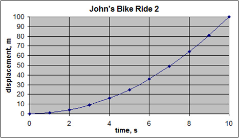
You can read right off the graph that John's displacement at 5 s is 25 m. In addition, notice that under constant acceleration, the graph of displacement vs. time is a parabola. Remember that the equation that describes displacement vs. time is quadratic: Δd = viΔt + ½ a(Δt)2. This graph shows a parabola that opens up. If the acceleration were negative, the parabola would open down.